Simple Image saliency detection from histogram backprojection

Image saliency detection is about identifying the interesting parts of an image, the parts of the image human eyes would fix on.

Saliency detection is used in a lot of applications, the most popular of them is probably automatic thumbnail generation, where a descriptive thumbnail has to be generated for an image.
Usually a saliency map is generated, where a pixel is bright if it’s salient, and dark otherwise.
There are lots of interesting papers on this. Check out a great overview on saliency detection.
Anyway, in this post I’l share a simple heuristic for saliency detection.
The basic idea is that usually salient pixels should have very different colors than most of the other pixels in the image.
We measure each pixel’s similarity to the background by histogram back-projection.
Finally, we refine the saliency map with Grabcut.
So here we go.
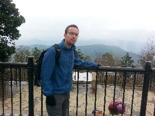
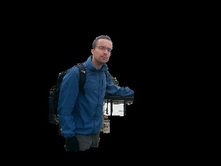
Original image (taken at Mount. Takao, Japan)

1. Preprocessing: Filter the image with Mean Shift for an initial soft segmentation of the image.

This groups together close pixels that are similar, and generates a very smooth version of the image.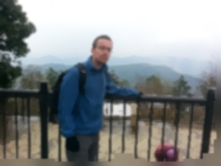

Some of the saliency papers call an inital segmentation stage - “abstraction”.
It’s common that each segment is compared somehow to other segments to give it a saliency score.
We won’t do that here, though.
For speed we use the multiscale pyramidal meanshift version in OpenCV.
This stage isn’t entirely necessary, but improves results on some images.

cv2.pyrMeanShiftFiltering(img, 2, 10, img, 4)

2. Back-project the Hue, Saturation histogram of the entire image, on the image itself.

The back-projection for each channel pixel is just the intensity, divided by how many pixels have that intensity.
It’s an attempt to assign each pixel a probability of belonging to the background.
We use only 2 bins for each channel.
That means we quantize the image into 4 colors (since we have 2 channels).
The more levels we use, the more details we get in the saliency map.

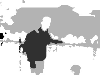
Notice how the blue jacket gets low values, since it’s unique and different from the background.
Also notice how the face back-projection is not unique.
That’s bad, we will try to fix that later.

def backproject(source, target, levels = 2, scale = 1):
    hsv = cv2.cvtColor(source,  cv2.COLOR_BGR2HSV)
    hsvt = cv2.cvtColor(target, cv2.COLOR_BGR2HSV)
    # calculating object histogram
    roihist = cv2.calcHist([hsv],[0, 1], None, [levels, levels], [0, 180, 0, 256] )

    # normalize histogram and apply backprojection
    cv2.normalize(roihist,roihist,0,255,cv2.NORM_MINMAX)
    dst = cv2.calcBackProject([hsvt],[0,1],roihist,[0,180,0,256], scale)
    return dst

backproj = np.uint8(backproject(img, img, levels = 2))

3. Process the back-projection to get a saliency map.

So here we smooth the back-projection image with mean shift, enhance the contrast of the saliency map with histogram equalization, and invert the image.
The goal is to produce a smooth saliency map where salient regions have bright pixels.

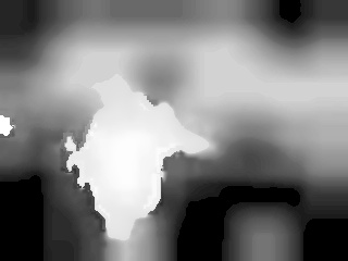
cv2.normalize(backproj,backproj,0,255,cv2.NORM_MINMAX)

saliencies = [backproj, backproj, backproj]
saliency = cv2.merge(saliencies)
cv2.pyrMeanShiftFiltering(saliency, 20, 200, saliency, 2)
saliency = cv2.cvtColor(saliency, cv2.COLOR_BGR2GRAY)
cv2.equalizeHist(saliency, saliency)

4. Threshold.

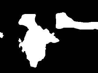
Ok, we have a few issues here:
- The segmentation is pretty rough.
- My head isn’t attached to the salient region.

(T, saliency) = cv2.threshold(saliency, 200, 255, cv2.THRESH_BINARY)

5. Find the bounding box of the connected component with the largest area.

We now have two salient regions.
A heuristic we use here is that the salient object will probably be the largest one.
We could’ve similarly assumed that the salient object will usually be closest to the center.
Saliency papers call that “encoding a prior”, since we use prior knowledge about how salient objects look.

def largest_contour_rect(saliency):
    contours, hierarchy = cv2.findContours(saliency * 1,
    cv2.RETR_LIST,cv2.CHAIN_APPROX_SIMPLE)

    contours = sorted(contours, key = cv2.contourArea)
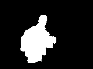
    return cv2.boundingRect(contours[-1])

6. Refine the salient region with Grabcut.

We use the bounding box as an initial foreground estimation, and apply Grabcut.
This makes the salient region segmentation much more accurate,
and most importantly, attaches back my head.

def refine_saliency_with_grabcut(img, saliency):
    rect = largest_contours_rect(saliency)
    bgdmodel = np.zeros((1, 65),np.float64)
    fgdmodel = np.zeros((1, 65),np.float64)
    saliency[np.where(saliency > 0)] = cv2.GC_FGD
    mask = saliency
    cv2.grabCut(img, mask, rect, bgdmodel, fgdmodel, 1, cv2.GC_INIT_WITH_RECT)
    mask = np.where((mask==2)|(mask==0),0,1).astype('uint8')
    return mask

Link to the code on github.
I like this method since it’s simple, but it has it’s drawbacks.